Neural networks and transformers - Notions
[IN PROGRESS]
Perceptron
Mark I Perceptron machine, the first implementation of the perceptron algorithm.
A perceptron is the simplest form of a feedforward neural network - it's a single artificial neuron that takes input features, multiplies each by a weight, adds a bias term, and applies a step function to output a binary decision (like classifying if a point is above or below a line).
Neural networks, MLPs
Inspired by the human brain, a neural network is a layered system of artificial neurons that processes information by combining input features with learned weights at each layer.
The Multi-Layer Perceptron (MLP)
Each neuron computes a weighted sum of its inputs and applies a non-linear activation function (like ReLU or sigmoid), allowing the network to learn complex patterns by transforming features into increasingly abstract representations.
This figure illustrates a multi-layer perceptron (or MLP) with two hidden layers. An MLP is a fully connected feed-forward neural network made up of perceptrons. Fully connected means any given perceptron of any given layer (except the first layer) is connected to all perceptrons of the previous layer. Feed-forward means there's a clear ordering of layers and connections occur only between consecutive layers. Intermediate layers are called hidden layers, and its perceptrons hidden units. The number of units in the first and last layers depend on the application. The number of units on each hidden layer, as well as the number of hidden layers, are design choices.
A Convolutional Neural Network (CNN), to classify images into one of 3 classes: Horse, Zebra or Dog.
Through training with backpropagation and gradient descent, the network iteratively adjusts its weights to minimize prediction errors, enabling it to automatically learn powerful mappings from raw inputs (like pixels or words) to desired outputs (like object categories or translations).
Activation functions
Just like biological neurons that either fire or stay quiet based on their input, artificial neurons need a way to decide whether and how strongly to activate. This is the role of activation functions.
Activation functions introduce non-linearity into neural networks - without them, even deep networks would just compute fancy linear combinations. ReLU (Rectified Linear Unit) simply outputs the input if positive and zero otherwise, while sigmoid squishes inputs into values between 0 and 1. Despite ReLU's simplicity, it usually works better than sigmoid or tanh for deep networks.
The final layer typically uses task-specific activations: softmax for converting raw scores into probabilities (classification), or linear for regression problems.
Loss functions
The loss function measures how wrong a neural network's predictions are. For classification, cross-entropy loss measures how far predicted probabilities are from the true labels, while mean squared error is commonly used for regression to measure the average squared difference between predictions and true values.
This is what the network tries to minimize during training: make better predictions, get a lower loss score. The choice of loss function depends on the task and effectively tells the network what "better" means.
Gradient descent
Gradient descent is an optimization algorithm that aims to find the minimum value of an error function.
It is like trying to find the lowest point in a valley (the error landscape) while blindfolded, where each step is taken in the direction that feels steepest downhill. Though sometimes you might get stuck in a small dip (local minimum) that isn't actually the deepest valley.
Through many small steps and using techniques to escape these local minima, it gradually reaches a global minimum where the error is lowest, finding the best solution to problems like fitting machine learning models to data.
Back propagation
Backpropagation figures out how much each connection in a neural network needs to be adjusted to reduce prediction errors.
Starting from the final error, it works backwards through the network to calculate how responsible each connection was for the mistakes, just like tracing back a path of wrong turns.
These calculations tell gradient descent exactly how to adjust the network's connections to make better predictions next time.
The training chain
Neural networks learn through a repeating cycle of prediction, evaluation, and improvement. This cycle has four key steps:
Forward pass: the network processes input data through its layers, applying weights and activation functions to make predictions
Loss calculation: the loss function (like cross-entropy) measures how wrong these predictions are compared to the true answers
Backpropagation: working backwards through the network, backprop calculates how much each weight contributed to the error
Parameter update: gradient descent uses these calculations to adjust the weights, slightly improving the network's predictions
Optimizers
While basic gradient descent gets the job done, modern neural networks use smarter optimizers that adapt how big each weight update should be.
Adam, the most popular optimizer, maintains separate learning rates for each weight and adapts them based on recent gradients. SGD (Stochastic Gradient Descent) with momentum remembers previous update directions to avoid zigzagging, like a ball rolling downhill. These tricks help networks train faster and often find better solutions than simple gradient descent.
The choice of optimizer and its settings (learning rate, momentum, etc.) can make the difference between a network that learns well and one that struggles to improve.
Transformers
The legendary paper (here) that introduced the transformer architecture.
The transformer architecture, like in the Attention is all you need paper, with an encoder and a decoder (as it was for translation). GPT-like models are decoder-only transformers.
The original GPT architecture
Attention
The attention mechanism
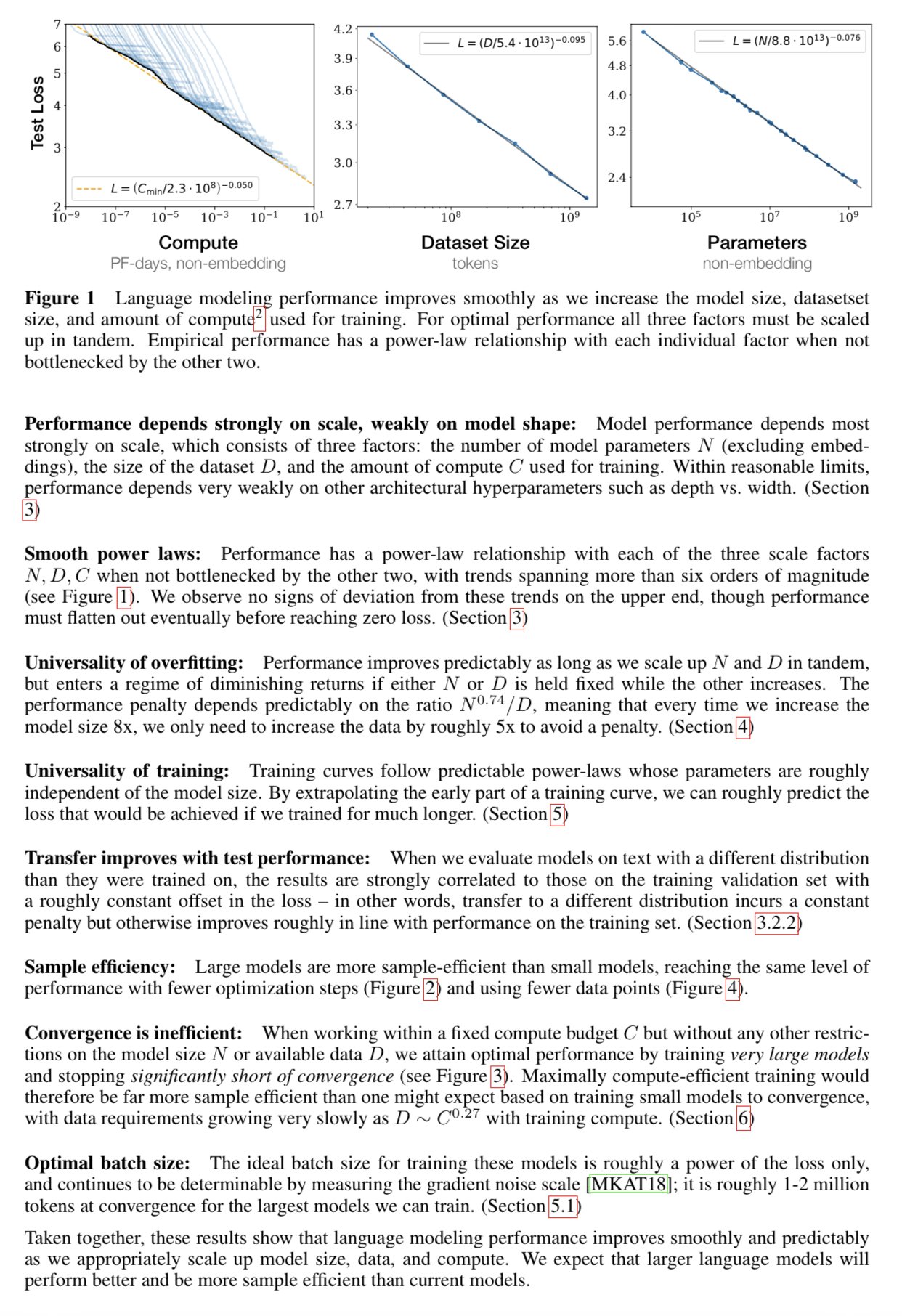
Scaling laws
Train a bigger model, on a bigger dataset, with more compute -> Better model
Scaling laws paper (here), applicable for the training of transformer language models.
Inference-time compute
With o1 we have a new scaling law, at inference:
More compute for inference -> Better results


